Regression Analysis Paper Example: Determinants of Female Headed Households

In the traditional setting, households were largely headed by men. However, in the recent past, there has been increasing number of women headed household, more so in highly modernized and developed economies. This study relied on cross-country data to examine possible predictors of the number of female headed houses. A regression analysis was used to examine the direction and strength of the association as well as the regression equation to predict the relationship. Key independent variables applied included: GDP, female labor participation and divorce.

Results

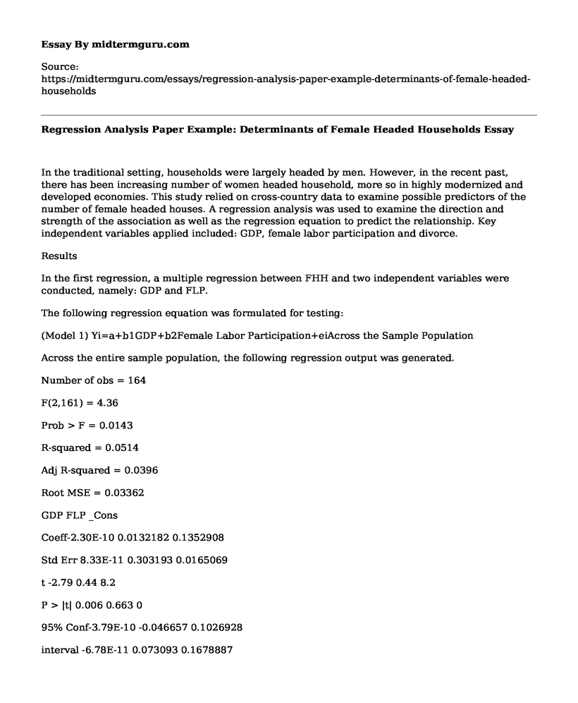
In the first regression, a multiple regression between FHH and two independent variables were conducted, namely: GDP and FLP.

The following regression equation was formulated for testing:

(Model 1) Yi=a+b1GDP+b2Female Labor Participation+eiAcross the Sample Population

Across the entire sample population, the following regression output was generated.

Number of obs = 164

F(2,161) = 4.36

Prob > F = 0.0143

R-squared = 0.0514

Adj R-squared = 0.0396

Root MSE = 0.03362

GDP FLP _Cons

Coeff-2.30E-10 0.0132182 0.1352908

Std Err 8.33E-11 0.303193 0.0165069

t -2.79 0.44 8.2

P > |t| 0.006 0.663 0

95% Conf-3.79E-10 -0.046657 0.1026928

interval -6.78E-11 0.073093 0.1678887

From the result, a negative association exists between GDP and the number of FHH (r=-2.30E-10) and the association is significant (p=0.006, so <0.05). From the regression equation, -squared = 0.0514, suggesting that about 5% of the variation in the number of FHH is accounted for by the GDP and FLP, and taking into account other influencing factors, two factors accounts for 3.96 % of the variation in FHH (Adj R-squared = 0.0396).

However, there is a positive statistical association between FHH and FLP, since r=0.0132182. The association is, however, insignificant (p= 0.663, >0.05). Comparing the two, GDP is a stronger determinant. From the above values, the following regression equation can be formulated:

FHH=0.1352908+(-2.30E-10GDP)+0.0132182Female Labor Participation+eiAmong Various Income Groups

Low Income Province

The regression output among the low income groups is summarized in the table below:

Group=0 (low income province)

Number of obs = 84

F(2,81) = 3.31

Prob > F = 0.0417

R-squared = 0.0754

Adj R-squared = 0.0526

Root MSE = 0.03322

GDP FLP _Cons

Coeff-9.33E-11 0.1212312 0.0851362

Std Err 6.26E-10 0.0481349 0.030036

t -0.15 2.52 2.83

P > |t| 0.882 0.014 0.006

95% Conf-1.34E-09 0.0254578 0.0253739

interval 1.15E-09 0.2170046 0.1448985

The results for this group is nearly similar with the entire group. A negative insignidficant association exists between GDP and the number of FHH (r=-9.33E-11, p= 0.882). From the regression equation, -squared = 0.0754, suggesting that about 7.54% of the variation in the number of FHH is accounted for by the GDP and FLP, and taking into account other influencing factors, GDP and FLP accounts for 5.26% of the variation in FHH (Adj R-squared = 0.0526).

However, there is a positive significant statistical association between FHH and FLP, since r=0.1212312. Comparing the two, FLP is a stronger predictor of FHH, as it has a higher co-efficient and the association is significant (p=0.014, i.e.<0.05). From the above values, the following regression equation can be formulated:

FHH=0.1352908-9.33E-11GDP)+0.1212312Female Labor Participation+eiHigh Income Province

Group=1 (high income province)

Number of obs = 80

F(2,77) = 1.21

Prob > F = 0.3039

R-squared = 0.0305

Adj R-squared = 0.0053

Root MSE = 0.02959

GDP FLP _Cons

Coeff-7.24E-11 -0.050006 0.1495691

Std Err 8.70E-11 0.0342453 0.0190943

t -0.83 -1.46 7.83

P > |t| 0.408 0.148 0

95% Conf-2.46E-10 -0.1181972 0.1115475

interval 1.01E-10 0.0181851 0.1875906

From the result, a negative association exists between GDP and the number of FHH (-7.24E-11), but the association is insignificant (p=0.408 , p>0.05). From the regression equation, R-squared = 0.0305, suggesting that about 3.05% of the variation in the number of FHH is accounted for by the GDP and FLP, and taking into account other influencing factors, GDP and FLP accounts for 2.956 % of the variation in FHH (Adj R-squared = 0.02959).

There is also a negative statistical association between FHH and FLP, since r=-0.050006. Again, the association is insignificant (p =0.148, >0.05). From the above values, the following regression equation can be formulated:

FHH=0.1495691+(-7.24E-11GDP)+(-0.050006)Female Labor Participation+eiModel 2

This model was developed by undertaking multiple regression of FHH against three variables, namely: GDP, FLP and number of divorced women. The model regression equation is as below:

Model 2 Yi=a+b1GDP+b2Female Labor Participation+b3Divorced+eiNumber of obs = 164

F(3,160) = 40.42

Prob > F = 0.0000

R-squared = 0.4311

Adj R-squared = 0.4205

Root MSE = 0.02612

GDP FLP Divorced _Cons

Coeff-1.39E-10 0.064329 3.183536 0.0333792

Std Err 6.53E-11 0.0240665 0.3080565 0.0161765

t -2.13 2.67 10.33 2.06

P > |t| 0.034 0.008 0 0.041

95% Conf-2.68E-10 0.168001 2.575155 0.0014322

interval -1.04E-11 0.1118579 3.791917 0.653261

From the results, all the variables have a significant association with FHH (p<0.05 in all cases). There is a negative association with GDP (r=-1.39E-10), but a positive association with FLP (r=0.064329) and number of divorced population (r=3.183536). Of the three variables, the number of divorced population is the strongest predictor (p=0, and r is the highest of the three independent variables). Taking together the three factors, they account for about 42.05% of the variation in the FHH (Adj R-squared = 0.4205)

Low income ProvinceGroup=0 (low income province)

Number of obs = 84

F(3,80) = 14.97

Prob > F = 0.0000

R-squared = 0.3595

Adj R-squared = 0.3355

Root MSE = 0.02782

GDP FLP Divorced _Cons

Coeff1.70E-10 0.1358026 2.413936 0.0123656

Std Err 5.26E-10 0.403871 0.4052469 0.0279648

t 0.32 3.36 5.96 0.44

P > |t| 0.747 0.001 0 0.66

95% Conf-8.78E-10 0.0554296 1.607469 -0.0432861

interval 1.22E-09 0.2161755 3.220403 0.0680172

Among this group, all the factors have a positive association with FHH, through the association with GDP is insignificant (p=0.747) while in the rest it is significant.

High Income Province

Group=1 (high income province)

Number of obs = 80

F(3,76) = 24.47

Prob > F = 0.0000

R-squared = 0.4913

Adj R-squared = 0.4712

Root MSE = 0.02158

GDP FLP Divorced _Cons

Coeff-9.85E-11 0.0428588 4.25442 0.0162393

Std Err 6.35E-11 0.0273612 0.5127099 0.0212598

t -1.55 1.57 8.3 0.76

P > |t| 0.125 0.121 0 0.447

95% Conf-2.25E-10 -0.0116357 3.23327 -0.0261034

interval 2.80E-11 0.0973533 5.27557 0.0585819

Among this group, a negative insignificant association exists between FHH and GDP (r=-9.85E-11 , p=0.125). A positive insignificant association exists between FHH and FLP (r=0.0428588, p=0.121) while number of divorced has a significant association positive association (r=4.25442, p=0).These results affirm that divorce is the strongest predictor of FHH among the three.

Model 3

This model considers GDP, FLP and the number of married . It is depicted by the model below/l

Model 3 Yi=a+b1GDP+b2Female Labor Participation+b3Married+eiNumber of obs = 164

F(3,160) = 40.05

Prob > F = 0.0000

R-squared = 0.4289

Adj R-squared = 0.4182

Root MSE = 0.02617

GDP FLP Married _Cons

Coeff-1.47E-10 0.0216411 -0.563434 0.4608149

Std Err 6.53E-11 0.023613 0.547896 0.0341628

t -2.24 0.92 -10.28 13.49

P > |t| 0.026 0.361 0 0

95% Conf-2.76E-08 -0.024993 -0.671638 0.3933467

interval -1.76E-11 0.0682749 -0.455229 0.528283

GDP and married negatively predicts FHH (r=-1.47E-10, and -0.563434 respectively). Married population is a greater predictor, though both have significant association with FHH (as p<0.05).

Low Income

Group=0 (low income province)

Number of obs = 84

F(3,80) = 12.68

Prob > F = 0.0000

R-squared = 0.3222

Adj R-squared = 0.2968

Root MSE = 0.02862

GDP FLP Married _Cons

Coeff8.63E-10 0.1110015 -0.4850397 0.3512173

Std Err 5.68E-10 0.0415131 0.0898693 0.0556788

t 1.52 2.67 -5.4 6.31

P > |t| 0.132 0.009 0 0

95% Conf-2.67E-10 0.0283879 -0.6638854 0.2404131

interval 1.99E-09 0.1936151 -0.3061941 0.4620216

Among this group, GDP and FLP positively predict FHH, but only FLP is a significant predictor (p=0.009). Married population is a negative significant predictor (r=-0.4850397, p=0).

High Income

Group=1 (high income province)

Number of obs = 80

F(3,76) = 28.91

Prob > F = 0.0000

R-squared = 0.5329

Adj R-squared = 0.5145

Root MSE = 0.02067

GDP FLP Married _Cons

Coeff-1.19E-10 -0.0249098 -0.6057821 0.5045856

Std Err 6.10E-11 0.0240848 0.0669932 0.0414654

t -1.96 -1.03 -9.04 12.17

P > |t| 0.054 0.304 0 0

95% Conf-2.41E-10 -0.0728788 -0.7392106 0.4220001

interval 2.14E-12 0.0230592 -0.4723535 0.5871712

Among this group, GDP, married and FLP are all negatively associated with FLP, but only married is a significant predictor because p>0.05 for the GDP and FLP.

Conclusion

GDP, FLP, number of divorced and number of married population predict FHH. However, the nature of association varies depending on the economic status.